Paper: arXiv:2610.35781.
The previous post on this blog ended with a negative result and a list of open routes. The six standard Strang splittings of kinetic Langevin dynamics, OBABO and BAOAB among them, are not accelerated from cold starts: with step size and friction fixed from the curvature bounds and the dimension alone, no mixing time bound of order √κ holds over the smooth strongly convex class. Whether acceleration is possible for an implementable scheme, by warm starts, dynamic tuning, randomized integrators or Metropolis adjustment, was left open.
The new preprint takes the last route, together with a warm start. It proves that Metropolis-adjusted OBABO mixes in a number of gradient evaluations of order √κ, up to the dimension and logarithms, provided the accept/reject decision uses a uniform random number that is updated non-reversibly across steps, as proposed by Neal, instead of being redrawn at every step. This post describes the sampler, the identity that makes the persistent uniform effective, the two main theorems, and the structure of the proof.
1. The acceleration question for adjusted samplers
Fix a target μ_target(dx) ∝ exp(−U(x)) dx on ℝ^d and consider kinetic Langevin dynamics,
dX_t = V_t dt, dV_t = −∇U(X_t) dt − γ V_t dt + √(2γ) dW_t,
with invariant measure μ = μ_target ⊗ N(0, I_d). Throughout, m I ⪯ ∇²U ⪯ L I, and κ = L/m is the condition number. With friction γ = 2√m the dynamics converge to μ at a rate of order √m, independently of L: in L²(μ) by Cao, Lu and Wang, and in relative entropy by Lu. Since the stability of an explicit Verlet-based discretization requires a step of order L^(−1/2), a discretization that inherited this rate would reach accuracy ε after of order √κ log(1/ε) gradient evaluations, ignoring the dependence on d, against κ log(1/ε) for overdamped samplers. This is the sense of acceleration used here, by analogy with Nesterov’s method in optimization. It is also the best one can hope for: for centered Gaussian targets, sampling to a fixed small total variation error requires in the worst case at least of order min(√κ, d) evaluations of U and ∇U (Chewi, de Dios Pont, Li, Lu and Narayanan).
For Metropolis-adjusted samplers, the known bounds on the full class of strongly log-concave targets were linear in κ or worse. The bounds of Lee, Shen and Tian and of Wu, Schmidler and Chen for MALA depend linearly on κ, and the coupling bound of Bou-Rabee and Oberdörster for adjusted OABAO carries a factor κ^(3/2). Apers, Gribling and Szilágyi obtained √κ d^(1/4) on Gaussian targets, with a proof that relies on Gaussian structure.
Question. Is there a Metropolis-adjusted discretization of kinetic Langevin dynamics that reaches a fixed total variation accuracy from a warm start after a number of gradient evaluations of order √κ, up to the dimension and logarithms, for every target in the smooth strongly log-concave class?
The answer given in the preprint is yes, for OBABO, under an additional Lipschitz condition on the Hessian, once the accept/reject uniform is updated non-reversibly.
2. Adjusted OBABO with a non-reversibly updated uniform
OBABO with step size h applies, in this order, a half-step of the Ornstein-Uhlenbeck flow of the velocity, a half kick by the force, a free flight, a half kick, and a second Ornstein-Uhlenbeck half-step:
O_s(x, v) = (x, e^(−γs) v + (1 − e^(−2γs))^(1/2) ξ), B_s(x, v) = (x, v − s∇U(x)), A_s(x, v) = (x + sv, v).
The three middle steps form the velocity Verlet integrator Φ = B_(h/2) ∘ A_h ∘ B_(h/2). The adjusted chain proposes Φ(w) from the state w after the first noise half-step, accepts the proposal or reverses the velocity, and then applies the second noise half-step. Write H(x, v) = U(x) − min U + |v|²/2 and ΔH(w) = H(Φ(w)) − H(w) for the energy error of the proposal, and h̄ = h√L for the dimensionless step size.
Writing the uniform random number of the Metropolis test as u = exp(−ℓ), the test accepts exactly when ℓ > ΔH. The standard rule draws a fresh exponential ℓ at every step. Neal’s non-reversibly updated uniform keeps ℓ from step to step and updates it on acceptance: in terms of u this is u ← u e^(ΔH), and in terms of ℓ,
ℓ ← ℓ − ΔH on acceptance, ℓ unchanged on rejection.
The variant analyzed in the preprint runs N epochs of E consecutive steps, drawing ℓ once at the start of each epoch.
Definition (adjusted OBABO with a non-reversibly updated uniform). One epoch from z draws ℓ ~ Exp(1) independently of the past and then, for k = 0, …, E − 1, with w = O_(h/2)(z): sets (z, ℓ) ← (O_(h/2)(Φ(w)), ℓ − ΔH(w)) if ℓ > ΔH(w), and (z, ℓ) ← (O_(h/2)(S(w)), ℓ) otherwise, where S(x, v) = (x, −v) is the velocity reversal.
Each step costs one gradient evaluation. Invariance follows from the auxiliary-variable involution framework of GIST, with ℓ as the auxiliary variable: on ℝ^(2d) × (0, ∞), the map that sends (w, ℓ) to ((S∘Φ)(w), ℓ − ΔH(w)) when ℓ > ΔH(w), and leaves (w, ℓ) unchanged otherwise, is a volume-preserving involution that conserves the extended energy H + ℓ. So each step preserves μ ⊗ Exp(1), and each epoch preserves μ.
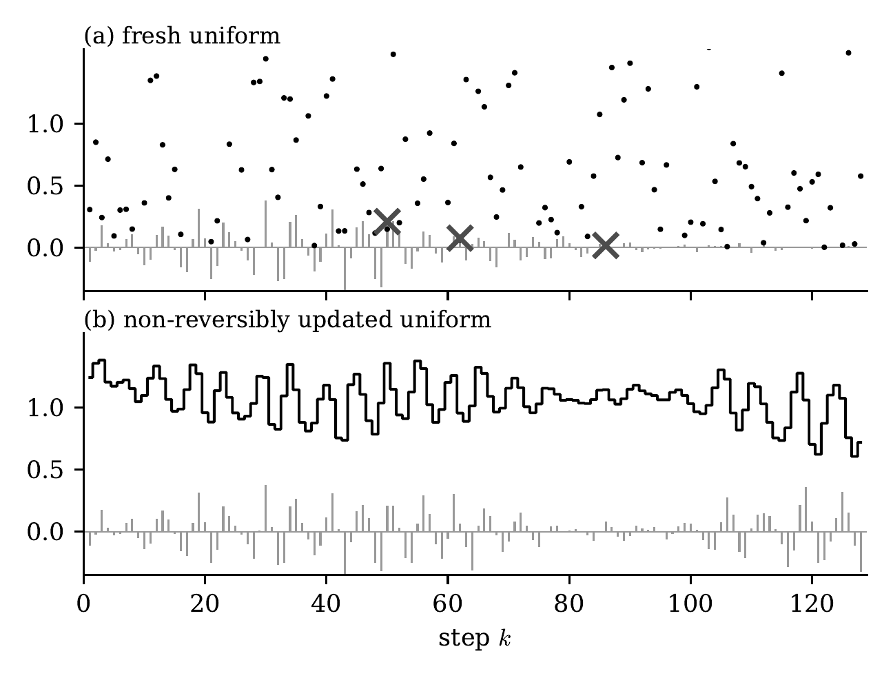
The figure compares the two rules along one run. With a fresh threshold the black dots are independent exponentials, and a rejection occurs whenever one falls below the gray bar. With the non-reversibly updated threshold the black line moves down by each accepted energy error and up when the error is negative. Its value before step k + 1 of an epoch is its initial value minus the sum of the energy errors accepted so far.
3. Telescoping energy errors
The reason the persistent threshold helps is an exact identity for the energy error of velocity Verlet. For a step from w = (x, v), let V = v − (h/2)∇U(x) be the velocity during the free flight and x_1 = x + hV the new position. Put
G(x) = (h²/8) |∇U(x)|², τ(w) = U(x_1) − U(x) − ⟨∇U(x) + ∇U(x_1), x_1 − x⟩/2,
so that τ is the error of the trapezoidal rule for U along the flight.
Lemma (energy error of velocity Verlet). For every w,
ΔH(w) = G(x_1) − G(x) + τ(w), |τ(w)| ≤ (h̄²/8) |V|², 0 ≤ G ≤ (h̄²/4)(U − min U).
If moreover ∇²U is L_H-Lipschitz, then |τ(w)| ≤ (L_H/12) h³ |V|³, and τ ≡ 0 when U is quadratic.
The Ornstein-Uhlenbeck half-steps do not move positions. Along a path X_0, X_1, … of the unadjusted chain, the partial sums of the energy errors therefore telescope:
S_n = ΔH_0 + … + ΔH_(n−1) = G(X_n) − G(X_0) + τ_0 + … + τ_(n−1).
Proposition (acceptance of every move of an epoch). Every move of an epoch is accepted if and only if ℓ > max_(1≤n≤E) S_n, and on this event the adjusted epoch coincides with the unadjusted chain driven by the same noises. Consequently
ℙ(a move of the epoch is rejected) = 𝔼[1 − exp(−max_n S_n⁺)] ≤ 𝔼[min(1, (h̄²/4) max_(n≤E) (U(X_n) − min U) + Σ_(k<E) |τ_k|)].
The leading part of the energy error enters only through a maximum over the visited positions, with no factor of E. With a fresh threshold at every step, the corresponding bound is Σ_(k<E) 𝔼[1 − exp(−ΔH_k⁺)], a sum of E terms whose positive parts do not cancel.
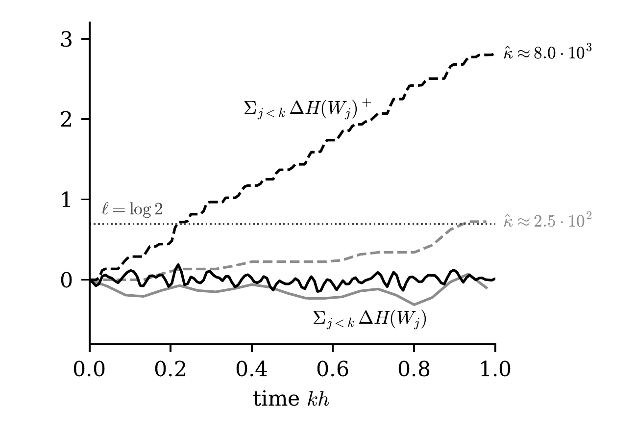
The figure shows both sums along one unit of time on the Sonar posterior. The accumulated signed error stays flat, well below the median of ℓ. The accumulated positive parts climb steadily and pass it. The same phenomenon is visible in the animation at the end of this post: the two chains reject the same fraction of moves, but the persistent threshold spends its rejections in bursts when it is nearly used up, and between bursts the chain runs for stretches of time without a rejection. Every rejection reverses the velocity, so a long rejection-free stretch is a stretch of ballistic motion along the slow directions of the target.
For a quadratic potential τ ≡ 0, and the rule takes a simple form. On acceptance ℓ drops by G(x_1) − G(x), and on rejection neither ℓ nor x changes, so ℓ + G(x) keeps its initial value ℓ_0 + G(x_0) throughout the epoch. The test ℓ > ΔH then reads G(x_1) < ℓ_0 + G(x_0). Within an epoch the adjusted chain is unadjusted OBABO confined to the ellipsoid {G < G(x_0) + ℓ_0}: a proposal that would leave it is rejected and the velocity reversed.
4. The main result
Let l_H = L_H / m^(3/2) be the scale-invariant Hessian-Lipschitz ratio, and let P denote the kernel of one epoch.
Theorem 1 (mixing of the adjusted chain). Assume m I ⪯ ∇²U ⪯ L I and that ∇²U is L_H-Lipschitz. Let ε ∈ (0, 1) and let ν be a probability measure with M_2 = ‖dν/dμ‖_(L²(μ)) < ∞. Put D = d + log(M_2/ε), Λ = log(2 + κ + l_H + D) and N = ⌈log(2/ε)/log 4⌉. There is an absolute constant C_0, and there are h̄ and E depending only on κ, l_H, d, M_2 and ε, such that
N E ≤ C_0 Λ^(3/2) (√(κD) + √(l_H) D^(3/4)) log(2/ε)
and ‖ν P^N − μ‖_TV ≤ ε.
A Gaussian centered within distance L^(−1/2) of the minimizer, with covariance (2L)^(−1) I, satisfies M_2 ≤ e (2κ)^(d/2), and such a point is found from any x_0 by Nesterov’s accelerated gradient method in O(√κ log(2 + κL|x_0 − x_*|²)) gradient evaluations. From this start the bound becomes
Õ(√(κd) + √(L_H) (d/m)^(3/4)),
where Õ hides logarithmic factors. The first term dominates when l_H ≤ κ/√d. This does not require U to be a small perturbation of a quadratic: it allows the Hessian to change by order L over a distance √(d/m), which is the largest scale of the position marginal.
The √κ dependence is necessary for this algorithm, already on Gaussian targets and from a warm start.
Proposition (sharpness in κ). Let d ≥ 2 and U(x) = (m/2) x_1² + (L/2)(x_2² + … + x_d²). Consider adjusted OBABO with any friction γ > 0 and any step size with h̄ < 2, using either a fresh uniform at every step or the non-reversibly updated uniform with any E. Start from μ(· | x_1 ≤ 0), whose density with respect to μ is at most 2. Then the position after n steps is at total variation distance greater than 1/4 from the position marginal of μ whenever
n < (√(2κ)/(4h̄)) (1 + h̄⁶/64)^((d−1)/2),
and hence, for every h̄ ∈ (0, 2), whenever n < (√2/8) √κ d^(1/6).
The proof combines a conductance bound for the half-space {x_1 ≤ 0} with an exact Gaussian integral that bounds the probability of an accepted crossing. At the step size of Theorem 1, which on this Gaussian is h̄ ≍ (DΛ)^(−1/2), the first condition requires n of order √(κDΛ), so there the term √(κD) is sharp up to logarithms. Over all step sizes, the dimension dependence on this family lies between d^(1/6) and d^(1/2).
5. Entropy decay of unadjusted OBABO
The proof of Theorem 1 rests on a contraction estimate for the unadjusted chain. Let K be the OBABO kernel, r = e^(−√m h) the velocity contraction factor of a noise half-step, and
λ = r²√m / (4(16 + r)) ≥ (√m/68) e^(−2√m h).
Theorem 2 (relative entropy decay of unadjusted OBABO). Assume m I ⪯ ∇²U ⪯ L I, that ∇²U is L_H-Lipschitz, γ = 2√m and √m h ≤ 3/16. Then for every z ∈ ℝ^(2d) and n ≥ 1,
KL(δ_z K^(n+1) ‖ μ) ≤ (17/15) e^(−λnh) [𝔼_z H(Z_1) + d log(κ / (2e h̄² (1 − √m h)))]
+ (16/15) [(h̄²/4) 𝔼_z (U(X_(n+1)) − min U) + sup_(1≤k≤n) ((L_H h²/(12λ)) 𝔼_z|V_k|³ + (221/(16r)) h̄² 𝔼_z|V_k|²)].
The rate involves no κ. The upper Hessian bound enters only through the factor h̄² of the bias, and L_H only through the third moment of the velocity. This is the discrete counterpart of Lu’s sharp entropic hypocoercivity estimate for the continuous dynamics. Lu’s functional is the relative entropy plus a multiple of the transport corrector
C(p) = 𝔼_p ⟨v, x − T(x)⟩,
where T is the Brenier map from the position marginal of p to the position marginal of μ. Its proof does not use an upper bound on the Hessian. Every step of it has an exact counterpart for OBABO except one: in the splitting the force acts impulsively at the two ends of a free flight, and the resulting mismatch in the time derivative of the corrector is the error of the trapezoidal rule applied to the differential entropy of the position marginal along the flight.
6. An entropy inequality for free transport
That trapezoidal error is controlled by the following inequality, which may be of independent interest.
Proposition (entropy inequality for free transport). Let X, V be random vectors in ℝ^d, let g be a nondegenerate Gaussian density on ℝ^d, and put
ℰ_g(t) = KL( Law(X + tV, V) ‖ Law(X + tV) ⊗ g ).
If ℰ_g(0) and ℰ_g(1) are finite, then ℰ_g(t) ≤ ℰ_g(0) + ℰ_g(1) for all t ∈ [0, 1].
The quantity ℰ_g(t) measures how far the velocity is from the reference Gaussian g, conditionally on the position, at time t of the free flight. The proposition says it cannot exceed the sum of its values at the two ends. The paper gives two proofs. The first adds Gaussian noise of variance t(1 − t) to the intermediate position X + tV = (1 − t)X + t(X + V), which gives the marginal at time t of a Brownian bridge from X to X + V, and applies strong subadditivity of entropy to the triple formed by the two endpoints and this point; the logarithmic terms in t(1 − t) cancel. It assumes finite second moments and finite differential entropy. The second is a dual argument that needs only the finiteness of ℰ_g(0) and ℰ_g(1).
The inequality is stated for a general pair (X, V) and does not see the potential. Combined with the exact one-step identities for the noise half-steps and the kicks, it gives a one-step decay of entropy plus a multiple of the corrector, and summation over steps gives Theorem 2.
7. From entropy decay to mixing
Theorem 2 controls the unadjusted chain; the adjusted chain is handled by a coupling of whole epochs.
Lemma (maximal endpoint coupling). There is a probability kernel (z, z̃) ↦ Γ_(z,z̃) to pairs of noise blocks for one epoch, with both marginals i.i.d. standard Gaussian, such that the unadjusted chains from z and z̃ driven by the two blocks differ at the end of the epoch with probability exactly ‖δ_z K^E − δ_(z̃) K^E‖_TV.
Run two copies of the adjusted chain, one from the initial distribution ν and one from the target distribution μ, use the same ℓ for both, and drive each epoch by noise blocks drawn from Γ. On the event that neither copy rejects a move, both coincide with their unadjusted chains, by the acceptance proposition of §3. So the copies differ at the end of the epoch with probability at most the total variation distance between the unadjusted endpoint laws plus the two rejection probabilities. The coupling is not adapted to the filtration of the chains: it is built on whole epochs, from the endpoints back to the noises. This is necessary. For Gaussian targets the meeting probability of any coupling of two copies of OBABO that acts step by step decays strictly more slowly than their total variation distance, as shown in joint work with Sonja Cox and Roy Schieven.
Proposition (coupling). Let 𝒟 be a measurable set of states and
q = sup_(z, z̃ ∈ 𝒟) ( ‖δ_z K^E − δ_(z̃) K^E‖_TV + β(z) + β(z̃) ),
where β(z) is the probability that an epoch from z rejects some move. Then for every N ≥ 1,
‖ν P^N − μ‖_TV ≤ q^N + N μ(𝒟^c) + M_2 (N μ(𝒟^c))^(1/2).
This is the localization idea of the earlier work with Oberdörster, in a form where the contraction is a total variation bound at the end of an epoch instead of a one-step Wasserstein contraction. No bound on the excursions of the adjusted chain is needed: under μ each epoch starts with law μ, so a union bound over epochs controls the probability of starting outside 𝒟, and the Cauchy-Schwarz inequality transfers this to the warm start.
To prove Theorem 1, take 𝒟 = {H ≤ R} with R of order D. For every z ∈ 𝒟 it then suffices that (i) the unadjusted epoch from z ends within a fixed small total variation distance of μ, and (ii) the adjusted epoch from z is rejection-free except with small probability. For (i), Theorem 2 gives relative entropy at most a constant after a physical time of order Λ/√m, that is E ≍ Λ√κ/h̄ steps, and Pinsker’s inequality converts this to total variation. For (ii), the acceptance proposition bounds the rejection probability by h̄² times the maximal energy along the epoch plus the accumulated τ, which is small for h̄ ≍ D^(−1/2). Then q ≤ 1/4, and N ≍ log(1/ε) epochs suffice.
Both steps need moments of the unadjusted chain over an epoch, including third moments of the velocity. Below a velocity v_* ≍ κ/(l_H h̄²), friction dominates the energy error of a Verlet step, and a Lyapunov function, the energy with a small twist ⟨x, v⟩, gives exponential moments for the chain stopped when it leaves this region. Above v_* there is no control uniform over the class. The argument of Theorem 2 is therefore applied to a comparison chain that reverses the velocity instead of making a flight faster than v_*. It coincides with the unadjusted chain except on an event whose probability is at most E times a quantity exponentially small in v_*², and the second term of Theorem 1 comes from the smaller step that the L_H terms force.
8. Bayesian logistic regression
The paper compares the two acceptance rules on Bayesian logistic regression posteriors with a Gaussian prior for the breast cancer and Sonar data sets, in the setup of Chopin and Ridgway. In the coordinates used there, m = 1, and the prior scale sets the condition number. The chain uses γ = 2 and redraws ℓ once per unit of time.
At a step based on the global bound L, h = h̄/√L with the practical value h̄ = 2/√(d + 2), both chains reject fewer than 0.2% of the moves for condition numbers from 11 to 1.9·10⁴, and the integrated autocorrelation time in units of time does not grow with κ. At these rejection rates the two rules give nearly the same chain.
The global bound L exceeds the largest Hessian eigenvalue L̂ at the mode by a factor 1.4 to 52, so this step is conservative. With h = 1/√L̂, outside the parameter range of Theorem 1, both chains reject about 7% to 13% of the moves, and the condition number at the mode κ̂ ranges from 9.5 to 9.5·10⁴ (breast cancer) and from 8 to 5.6·10⁴ (Sonar). The curvature varies along the chain, so the chains do not see a nearly Gaussian target.
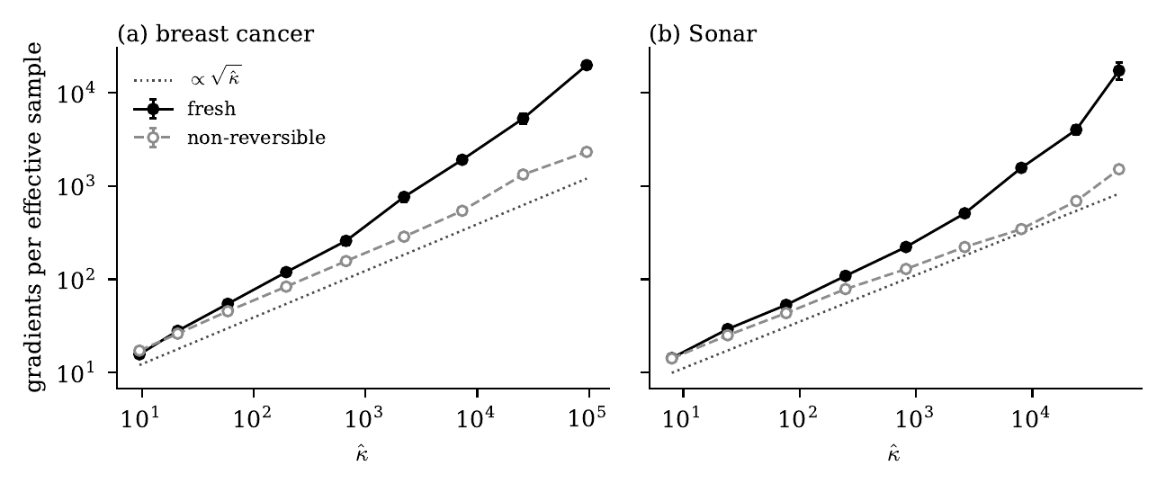
The integrated autocorrelation time of the chain with the non-reversibly updated uniform stays between about 4 and 8 units of time over these ranges, while that of the fresh-uniform chain grows from about 5 to 64 and 74. Least-squares fits of the logarithm of the cost against log κ̂ give slopes 0.54 ± 0.01 (non-reversibly updated) and 0.76 ± 0.02 (fresh) for breast cancer, and 0.50 ± 0.02 and 0.76 ± 0.05 for Sonar. The measured cost of the persistent chain grows like the square root of the condition number at the mode, beyond what Theorem 1 proves on this family, where the Hessian-Lipschitz constant grows like κ^(3/2) and the second term of the theorem gives κ^(3/4).
9. Scope and open problems
- The Hessian-Lipschitz condition. It enters only through the cubic bound on the trapezoidal error τ. Under strong convexity and a Lipschitz gradient alone the uniform bound is quadratic in h|V|, and this order is sharp, already in dimension one for a potential whose curvature jumps at the origin. Whether the chain itself needs a Lipschitz Hessian for square-root acceleration is open. A sharper rejection bound could exploit cancellation between signed errors, but must control their maximum partial sum over an epoch.
- Cold starts. Theorem 1 applies to any initial law with a finite L² density ratio. An accelerated bound for the adjusted chain started from an arbitrary point, without the optimization stage, is open. It is not expected in general: the attracting cycles behind the non-acceleration of the unadjusted splittings are the obstacle, though no such result is proved for the adjusted chain.
- Dependence on the dimension. On Gaussian targets the upper bound is √κ d^(1/2) and the lower bound √κ d^(1/6). Whether this chain attains √κ d^(1/4), as the proximal samplers of Chen, Chewi, Lu and Zhang and of Yuan, Guo and Chen do on the full class from a warm start, is open. It would require sharper control of rejection and larger steps.
- Other integrators. Theorem 2 is proved for OBABO. Whether an analogous entropy estimate yields accelerated mixing for other Metropolis-adjusted splittings, including OABAO with the non-reversibly updated uniform, is open.
The animation below runs both chains on the Sonar posterior at κ̂ = 5.6·10⁴ from the same start and with the same Gaussian noise. The top panel shows the coordinate along the smallest Hessian eigenvector at the mode, the middle panel the running density of that coordinate against a reference from a long independent run, and the bottom panel the share of run time spent in stretches between consecutive rejections longer than s.
Acknowledgements
Thanks to Bob Carpenter for introducing me to Neal’s non-reversibly updated accept/reject uniform, and to Pierre Monmarché for discussions on acceleration from cold and warm starts.
References
- Apers, S., Gribling, S., & Szilágyi, D. (2024). Hamiltonian Monte Carlo for efficient Gaussian sampling: long and random steps. Journal of Machine Learning Research, 25, Paper No. 348. DOI
- Bou-Rabee, N. (2026). Persistence Pays: square-root condition-number dependence for Metropolis-adjusted kinetic Langevin Monte Carlo with a non-reversibly updated accept/reject uniform. DOI
- Bou-Rabee, N. (2026). Provable non-acceleration of standard Strang splittings of kinetic Langevin dynamics. DOI
- Bou-Rabee, N., & Oberdörster, S. (2024). Mixing of Metropolis-adjusted Markov chains via couplings: the high acceptance regime. Electronic Journal of Probability, 29. DOI
- Bou-Rabee, N., Carpenter, B., & Marsden, M. (2026). GIST: Gibbs self-tuning for locally adaptive Hamiltonian Monte Carlo. Statistics Surveys, 20, 135–179. DOI
- Bou-Rabee, N., Cox, S., & Schieven, R. (2026). On couplings for kinetic Langevin diffusions. DOI
- Cao, Y., Lu, J., & Wang, L. (2023). On explicit L²-convergence rate estimate for underdamped Langevin dynamics. Archive for Rational Mechanics and Analysis, 247, Paper No. 90. DOI
- Chen, F., Chewi, S., Lu, J., & Zhang, M. S. (2026). Accelerated high-accuracy sampling from a warm start via the proximal bouncy particle sampler. DOI
- Chewi, S., de Dios Pont, J., Li, J., Lu, C., & Narayanan, S. (2024). Query lower bounds for log-concave sampling. Journal of the ACM, 71(4), Art. 29. DOI
- Chopin, N., & Ridgway, J. (2017). Leave Pima Indians alone: binary regression as a benchmark for Bayesian computation. Statistical Science, 32. DOI
- Lee, Y. T., Shen, R., & Tian, K. (2020). Logsmooth gradient concentration and tighter runtimes for Metropolized Hamiltonian Monte Carlo. In Proceedings of the 33rd Conference on Learning Theory. DOI
- Lu, J. (2026). A sharp hypocoercive entropy decay estimate for underdamped Langevin dynamics. DOI
- Neal, R. M. (2020). Non-reversibly updating a uniform [0,1] value for Metropolis accept/reject decisions. DOI
- Wu, K., Schmidler, S., & Chen, Y. (2022). Minimax mixing time of the Metropolis-adjusted Langevin algorithm for log-concave sampling. Journal of Machine Learning Research, 23, Paper No. 270. DOI
- Yuan, B., Guo, W., & Chen, Y. (2026). Reflected proximal dynamics for accelerated high-accuracy log-concave sampling. DOI